Name: Julien Bourgeois

This report covers two independent PyTorch experiments: a Fashion-MNIST classifier built from a multilayer perceptron, and an English–French translator that uses Bahdanau attention.

---

Part 1: Multilayer Perceptrons on Fashion-MNIST

The first experiment is a classification problem. Given a tiny grayscale picture of a clothing item, the model has to assign it to one of ten categories.

Task 1: Dataset and baseline model

Fashion-MNIST is a clothing-themed replacement for the original MNIST digit dataset: 70,000 images, each 28×28 and grayscale, with a single item roughly centered in the frame. The ten labels are T-shirt/top, Trouser, Pullover, Dress, Coat, Sandal, Shirt, Sneaker, Bag, and Ankle boot. Torchvision downloads the official 60,000 / 10,000 train/test split, and we hold out 10% of the official training set for validation, which leaves 54,000 images for training, 6,000 for validation, and 10,000 for test. Pixel intensities are scaled to the range [0, 1].

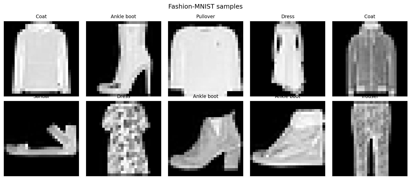
These are not photographs you would recognize at a glance. They are pixelated catalog thumbnails, and once a class name is printed above an image my brain fills in the rest, which is a kind of cheating: the label is already telling me what I am supposed to see. Cover the labels and the same pictures are much harder. Footwear still reads as shoes, and a heel is easy to separate from a sneaker, but coat versus pullover is genuinely difficult, dress versus coat is not much easier, and even pants are not obvious. If nobody had told me these were clothes, I could have talked myself into a completely different story. The model will not have that freedom, because it is only allowed to pick among those ten names.

The baseline is a multilayer perceptron. A fully connected layer is built to take a 1-D list of numbers rather than a 2-D grid, so we flatten each 28×28 picture into 784 values before the first linear layer. The architecture is flatten → Linear(784 → 256) → ReLU → Linear(256 → 10) logits, trained with SGD at learning rate 0.1, CrossEntropyLoss, batch size 256, and 10 epochs. There is no softmax on the last layer, because PyTorch’s CrossEntropyLoss expects raw logits and applies log-softmax internally; a softmax on the model would just duplicate that work. Torchvision only downloaded the images; the MLP started from random weights.

After 10 epochs the training loss was 0.380, the validation loss was 0.375, and validation accuracy was 0.868.

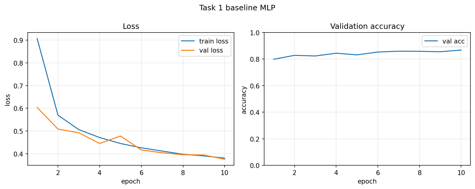
The validation curve bounced instead of tracking the training curve smoothly. At epoch 5 the validation loss actually got worse (0.478) before coming back down. The validation set is only 6,000 images, so that estimate is noisier than the training loss, and a learning rate of 0.1 is aggressive enough to produce an ugly epoch. Over the full run, validation drifted toward training rather than pulling away. That is not overfitting: validation never ran off while training kept falling. It is also not underfitting in the usual sense, since both losses came down and accuracy on held-out data improved.

That 87% also matches what looking at the pictures led me to expect. Footwear was already easy for a human, so I would guess the remaining mistakes are concentrated in lookalike tops — coat versus pullover, dress versus coat. We did not plot a confusion matrix, so that is a guess from the samples. Flattening throws away the 2-D layout on top of that, which means this network is not looking at a sleeve the way a person does; it is classifying a list of 784 pixel values. We already have 54,000 training images, so the limit here is more the model than the size of the dataset.

Task 2: Hidden layers and model capacity

I kept the same data, optimizer, loss, batch size, and 10 epochs, and only changed how much hidden capacity the MLP has.

Extra hidden layer (784 → 256 → 256 → 10)

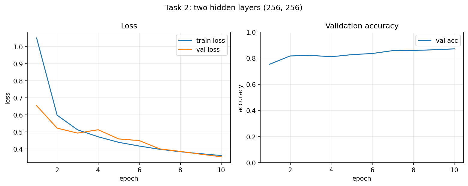
Adding a second 256-unit layer takes the network from about 204k parameters to about 269k. After 10 epochs the training loss was 0.361, the validation loss was 0.354, and validation accuracy was 0.871. That is three tenths of a point above the Task 1 baseline of 0.868, which on a 6,000-image validation set is about 18 extra correct labels. That is a wash, and I would not bother stacking the extra layer. It makes the model more complicated for no meaningful gain.

Validation still bumps — this time at epoch 4, when val loss rose from 0.493 to 0.513 while training kept falling — and then drifts back toward the training loss. Those wiggles are the same noisy validation estimate and the same aggressive learning rate as Task 1. Extra fully connected depth also does not restore the 2-D layout we flattened away, so the extra layer is still classifying a list of pixels.

One-neuron hidden layer (784 → 1 → 10)

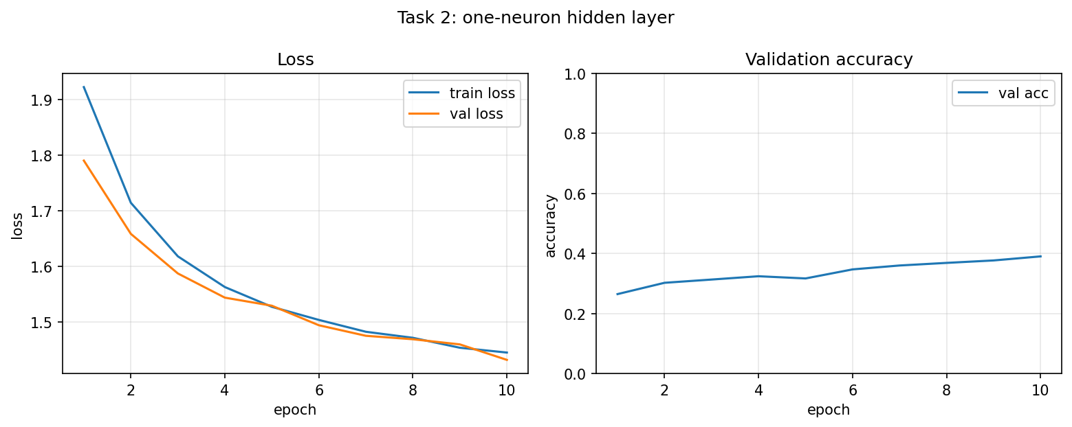
Here the hidden layer is a single neuron: 784 pixels are linearly combined into one number, ReLU is applied, and then ten class scores are read off that value. The whole network has 805 parameters. After 10 epochs the losses were still around 1.44, and validation accuracy was 0.390.

That one hidden value is one weighted sum of the whole picture, so the network has to line all ten classes up on a single axis. One number cannot separate coat from pullover, and it cannot even be trusted to keep shoe, shirt, and bag in different places if those classes overlap on that axis. Random guessing among ten balanced classes is 10%, so 39% means the tiny net did find some coarse signal — maybe how filled-in the thumbnail is, or footwear versus tops — but we did not inspect the weights, so that part is a guess. 39% is still far from the 87% of the 256-unit net, which is what you would expect if coat versus pullover is already hard when a person can see all 784 pixels.

The one-neuron curves were still drifting down at epoch 10, so a longer run might pick up a few more points. They will not close the gap to 87%. The losses never left the 1.4–1.9 range, which is a model that is too small, not one that just needed more epochs.

Task 3: Activation functions and gradients

I kept the two-layer width (256, 256) and only changed the activation after each linear layer: ReLU versus sigmoid. Same data, same SGD, same 10 epochs. An activation is what stops stacked linear layers from collapsing into one linear map. ReLU zeros negatives and leaves positives alone. Sigmoid squishes every number into (0, 1) with an S-curve whose two ends are almost flat.

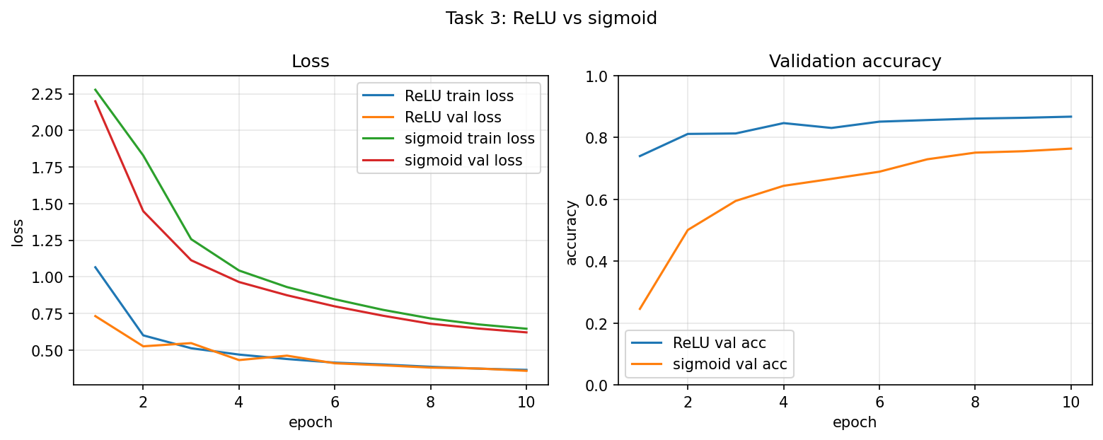
ReLU finished at train loss 0.364, val loss 0.357, and validation accuracy 0.868, the same neighborhood as Task 1. Sigmoid finished at 0.645 / 0.620 / 0.764. ReLU won this run. Sigmoid is still climbing at epoch 10, so it is not frozen at chance, but it started far behind — about 25% val accuracy at epoch 1 against ReLU’s 74% — and it never caught up. Swapping the activation dropped about ten points. Adding a ReLU layer in Task 2 had not.

The reason is how training actually updates the first layer, the one that sees the 784 pixels. Each update follows the gradient: if a weight barely changes the loss when you nudge it, it barely learns. On the flat parts of a sigmoid, that nudge does almost nothing, and those tiny factors multiply through a stack. The last hidden layer can still see a signal; the pixel layer gets starved. That is vanishing gradients. It is a learning bottleneck, not the size bottleneck from the one-neuron net.

The next two figures use a deeper net so that mechanism is easier to see: four hidden layers instead of two, random weights rather than a trained classifier, five minibatches, and the L2 gradient norm at each hidden layer. hidden_0 is closest to the pixels; hidden_3 is closest to the ten class scores. This is not another accuracy run.

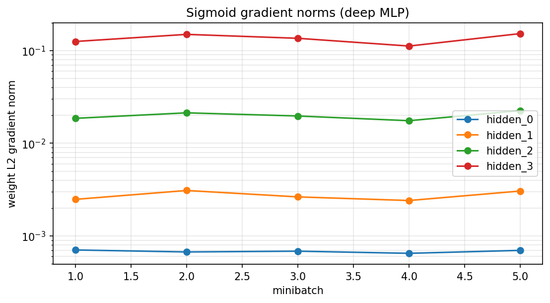
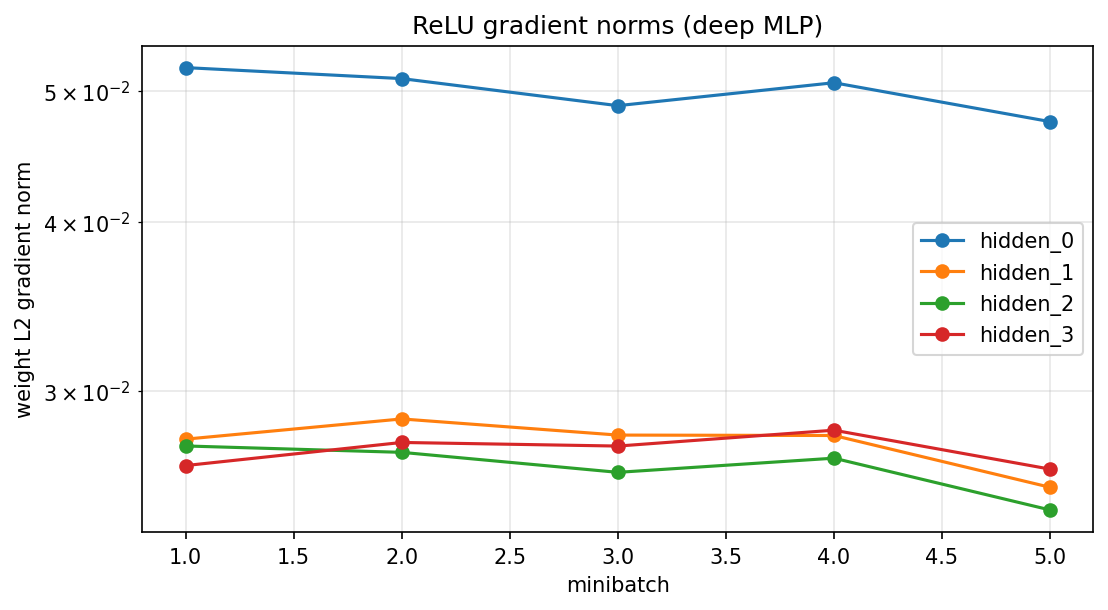
On the sigmoid plot (log scale) the last hidden layer sits around 0.14 and the first around 0.0007, roughly two hundred times smaller. The pixel layer is almost dead. On the ReLU plot the first layer is actually the largest, and the later layers stay in the same order of magnitude. ReLU does not squash everything onto a flat S, so a useful gradient can still reach the weights that look at the picture. That is why I would keep ReLU for this MLP, and why sigmoid lost the 10-epoch comparison even at only two hidden layers.

Task 4: Computational considerations

Training the MLP used more memory than classifying a new thumbnail with the finished weights.

The weights are needed in both phases: about 204k numbers in the Task 1 baseline, 269k with the extra hidden layer, and 805 in the one-neuron net. Prediction, with those weights frozen, does not need gradients, saved activations for backprop, or optimizer state. Our eval path is wrapped in torch.no_grad(), so PyTorch does not record a backward tape. It still computes hidden values for the current batch, then it can throw them away.

Training keeps extra copies. After a forward pass it stores activations so backprop can walk back through the net, and it stores a gradient for every weight — roughly another copy of the parameter tensor. Some optimizers also keep running buffers (momentum, Adam). Ours was plain SGD with no momentum, so we did not pay for those extra buffers, but the activation tape and the gradients are still there.

What actually grows with the experiment is the activation storage, not the 204k weights. A bigger batch means more images at once, so hidden activations are B × 256 instead of a small B. An epoch still sees each of the 54,000 images once; there are just fewer steps. Width and depth do the same thing: Task 2’s extra 256-unit layer is another full set of activations to keep, and the one-neuron net barely has a hidden tensor. These runs used MPS (the Mac GPU) when it was available, otherwise CPU.

---

Part 2: English–French translation with Bahdanau attention

The second experiment is translation: a short English sentence goes in, and the model writes French. This is an encoder–decoder with recurrent units and Bahdanau (additive) attention, not a Transformer. The encoder has no self-attention. It is a two-layer GRU that reads English tokens one by one and stores a vector at every position. The decoder has no causal attention mask and no target-side self-attention. It is a second two-layer GRU that writes one French token at a time. Causality comes from the GRU itself: each step only sees the previous hidden state and the previous token.

At each French step, Bahdanau attention scores every English position with score = v · tanh(W_q query + W_k key). The query is the decoder’s current hidden state (“what am I trying to say?”). The keys and values are the encoder outputs (“what did I read in English?”). Softmax turns those scores into weights that sum to one, and the context vector is the weighted sum of encoder states. Padding positions are masked to a large negative score before softmax so they do not get attention mass.

Training uses teacher forcing: the decoder is always fed the correct previous French word. At test time we greedy-decode: start from <bos>, always pick the highest-scoring next token, and stop at <eos> or a length cap. A wrong token is then fed back in, so errors can snowball. The data is the English–French pair file from D2L. Sentences are lowercased, punctuation is split off as its own token, and we keep pairs that fit in 16 tokens including specials. At most 12,000 pairs, with 10% held out for validation. Vocabularies are built on the training split only, min frequency 2, so rare words become <unk>. That left about 2,476 English types and 3,243 French types. Training uses Adam, batch size 64, 20 epochs, and gradient clipping at 1.0. Padding is ignored in the cross-entropy.

Task 1: Train the attention model

I trained two settings for 20 epochs. Depth stayed at two GRU layers, batch size 64, and max length 16. What changed was width, dropout, and learning rate.

Setting	Hidden / embed size	Dropout	Learning rate	Train loss	Val loss	Val BLEU
A	32	0.1	0.005	2.40	2.71	0.240
B	64	0.2	0.002	2.19	2.52	0.256

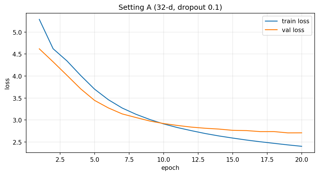
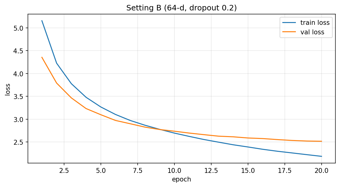
Train and validation loss are both teacher-forced token-level cross-entropy, so they are comparable to each other. BLEU is not: it is computed from greedy decoding with no gold previous token.

Both curves fall for the full 20 epochs. Early on, validation sits below training because dropout is on during training and off at eval, and because the training number averages a model that is still updating through the epoch. Around epoch 10 the lines cross. After that, training keeps falling faster than validation. A ends at 2.40 vs 2.71; B ends at 2.19 vs 2.52. That is a gap of about 0.3 in both runs. A’s validation is essentially flat for the last couple of epochs (2.7075 then 2.7086). B’s validation is still dropping at epoch 20. That is a little overfitting: the model is starting to fit the training sentences better than held-out ones. It is not a collapse. Validation never ran away upward while training fell.

B is better on every number: lower train loss, lower val loss, and BLEU 0.256 against 0.240. The main change is width (32 → 64). Extra units give the embeddings, the GRUs, and the attention projections more room. Dropout went up (0.1 → 0.2) and the Adam step went down (0.005 → 0.002), which should have made B harder to overfit, and the train–val gap is still about the same size as A’s. So the extra capacity is doing the work; the extra regularization did not erase the gain. I would keep B.

BLEU 0.25 is not a good translator. These sentences are short, the score is averaged sentence-level BLEU with add-one smoothing so zeros do not kill the log, and a 0.016 bump is small on a noisy metric. The example translations matter more.

English	Setting A	Setting B
go .	<unk> !	<unk> !
i lost .	je me suis senti .	j ‘ ai fait mon désaccord .
i’m ok .	j ‘ ai passé votre travail .	je suis heureux .
he is a teacher .	il est un homme .	il est très jolie .

Both settings turn go . into <unk> !. The English word go is common enough to be in the source vocabulary; the failure is on the French side. Rare French words were mapped to <unk> during training, so the decoder learned to emit <unk> as a real token. It guessed a command plus an exclamation mark and missed the verb.

The closest-to-French output is A’s il est un homme . for he is a teacher .: il/he and est/is are right, then it replaced teacher with man. B got il est and then wrote très jolie (very pretty), which is the wrong adjective and the wrong gender. The garbage example is i'm ok .: A produced j ' ai passé votre travail ., which is not even in the neighborhood, and B’s je suis heureux . has the right “I am …” shape with the wrong adjective. i lost . is similar: A said je me suis senti . (I felt), B wrote something that is not French for losing.

The model learned some local French patterns — il est, je suis, a period at the end — and it is not translating. That matches BLEU around 0.25 on this 12,000-pair subset.

Task 2: Visualize and interpret attention

The three heatmaps are from setting A, the same run as the example translations. Each row is one generated French token. Each column is one English token, including the source <eos>. Yellow means that French step put almost all of its attention on that English position; dark purple means almost none. A useful map would be roughly diagonal: il on he, est on is, the noun on teacher. Pads are already masked in the model, so these plots do not have a padding column. Mass on <eos> here is the real end-of-sentence token, not a dummy pad.

i'm ok . → j ' ai passé votre travail .

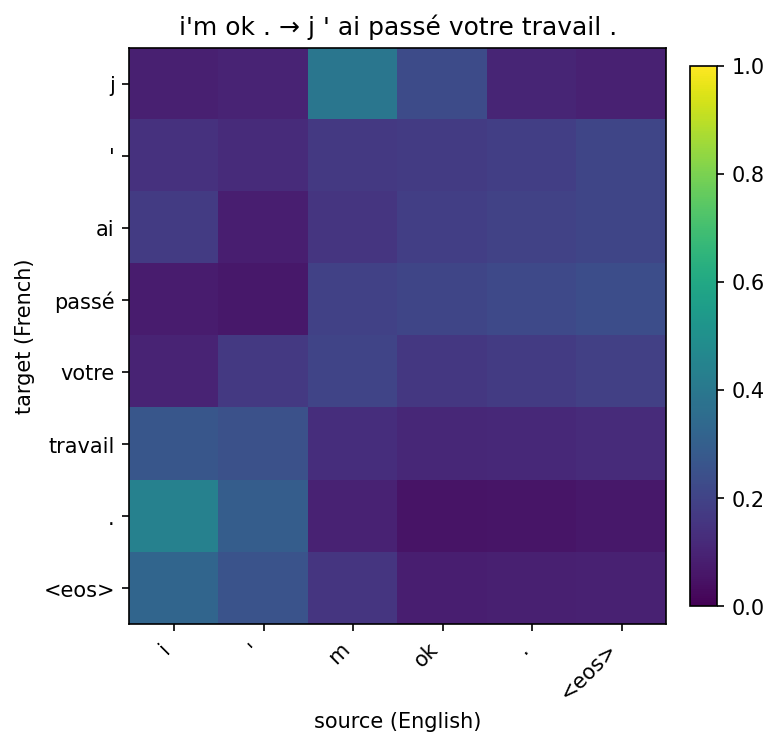
This map is unsuccessful. j (I) should look at i; it peaks on m (0.39) and then ok (0.23), with only 0.09 on i. The apostrophe and ai are almost uniform and both peak on source <eos>. passé also peaks on <eos> (0.24) instead of on ok. votre peaks on m. travail peaks on i (0.27). The period puts 0.44 of its mass on i and only 0.06 on the English period. Nothing in this map is reading ok as the word that needs a French equivalent. The decoder is emitting a French-looking sentence while looking at the contraction and the start of the sentence.

he is a teacher . → il est un homme .

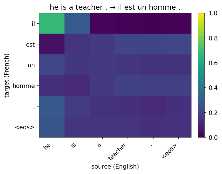
The first row is the helpful pattern. il puts 0.67 of its mass on he and 0.29 on is, and almost nothing on teacher or the period. That is the alignment you would want for a subject pronoun.

The rest of the map does not follow through. est should peak on is; after it avoids he, the row is almost flat, and the largest weight is source <eos> (0.21). un peaks on he (0.21) rather than on a (0.17). homme does put its largest weight on teacher (0.20), but that row is flat — a, the period, and <eos> are all around 0.19 — so it is not locked onto the noun. The model still wrote homme (man) instead of professeur. Attention on the right column is not enough if the next-token distribution prefers a more common word. The period and <eos> both go back to he.

i lost . → je me suis senti .

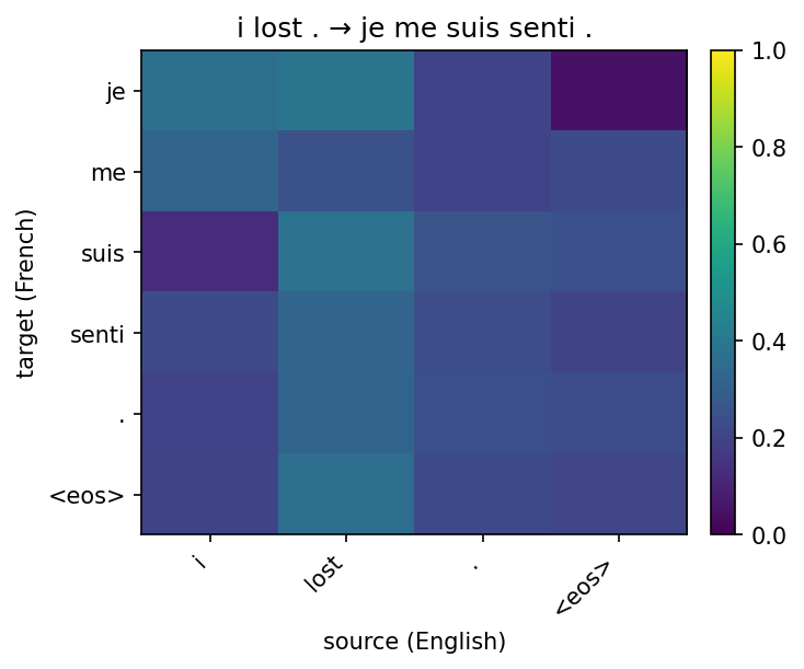
Almost every row after je piles onto lost. je is split between i (0.36) and lost (0.38). suis, senti, the period, and <eos> all peak on lost (0.32–0.37). Finding the only content word is better than the i'm ok map, but it is not a successful translation: the model built the reflexive je me suis senti (I felt) instead of something like j'ai perdu. Looking at lost and then saying senti means the attention is on the right column and the vocabulary choice is still wrong.

Helpful example: he is a teacher ., the il row. That is a real local alignment: the French subject pronoun attends to he.

Unsuccessful example: i'm ok .. The map is not diagonal, several rows park on source <eos>, the period attends to i, and no generated token treats ok as the thing to translate. i lost . is a second failure of a different kind: mass on lost without producing perdu.